Discussion of Supervised Approaches#
The previous example illustrates that we supervised training serves as a basis that can solve non-trivial tasks. The main workload is collecting a large enough data set of examples. Once that exists, we can train a network to approximate the solution manifold represented by these solutions, and the trained network can give us predictions very quickly. There are a few important points to keep in mind when using supervised training.

Some things to keep in mind…#
Natural starting point#
Supervised training is the natural starting point for any DL project. It really always makes sense to start with a fully supervised test using as little data as possible. This will be a pure overfitting test, but if your network can’t quickly converge and give a very good performance on a single example, then there’s something fundamentally wrong with your code or data. Thus, there’s no reason to move on to more complex setups that will make finding these fundamental problems more difficult.
Best practices 👑
To summarize the scattered comments of the previous sections, here’s a set of “golden rules” for setting up a DL project.
Always start with a 1-sample overfitting test.
Check how many trainable parameters your network has, and that your data is normalized properly.
Make sure the NN converges.
Then slowly increase the amount of training data (and potentially network parameters and depth).
Adjust hyperparameters (especially the learning rate).
Finally, introduce other components such as differentiable solvers or diffusion training.
Stability#
A nice property of the supervised training is also that it’s very stable. Things won’t get any better when we include more complex physical models, or look at more complicated NN architectures.
Thus, again, make sure you can see a nice exponential falloff in your training loss when starting with the simple overfitting tests. This is a good setup to figure out an upper bound and reasonable range for the learning rate as the most central hyperparameter. You’ll probably need to reduce it later on, but you should at least get a rough estimate of suitable values for \(\eta\).
Know your data#
All data-driven methods obey the garbage-in-garbage-out principle. Because of this it’s important to work on getting to know the data you are dealing with. While there’s no one-size-fits-all approach for how to best achieve this, we can strongly recommend to track a broad range of statistics of your data set. A good starting point are per quantity mean, standard deviation, min and max values. If some of these contain unusual values, this is a first indicator of bad samples in the data set.
These values can also be easily visualized in terms of histograms, to track down unwanted outliers. A small number of such outliers can easily skew a data set in undesirable ways.
Finally, checking the relationships between different quantities is often a good idea to get some intuition for what’s contained in the data set. The next figure gives an example for this step.
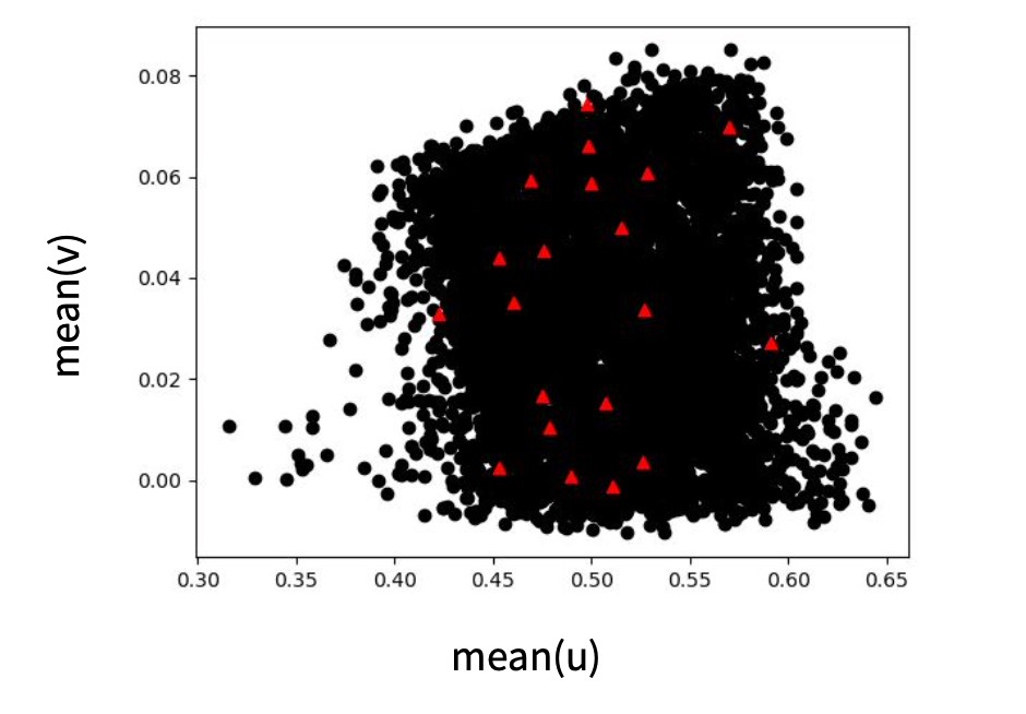
Fig. 12 An example from the airfoil case of the previous section: a visualization of a training data set in terms of mean u and v velocity of 2D flow fields. It nicely shows that there are no extreme outliers, but there are a few entries with relatively low mean u velocity on the left side. A second, smaller test data set is overlayed with red triangles, showing that its samples cover the range of mean motions well.#
Where’s the magic? 🦄#
A comment that you’ll often hear when talking about DL approaches, and especially when using relatively simple training methodologies is: “Isn’t it just interpolating the data?”
Well, yes it is! And that’s exactly what the NN should do. In a way - there isn’t anything else to do. This is what all DL approaches are about. They give us smooth representations of the data seen at training time. Even if we’ll use fancy physical models at training time later on, the NNs just adjust their weights to represent the signals they receive, and reproduce it.
Due to the hype and numerous success stories, people not familiar with DL often have the impression that DL works like a human mind, and is able to extract fundamental and general principles from data sets (“messages from god” anyone?). That’s not what happens with the current state of the art. Nonetheless, it’s the most powerful tool we have to approximate complex, non-linear functions. It is a great tool, but it’s important to keep in mind, that once we set up the training correctly, all we’ll get out of it is an approximation of the function the NN was trained for - no magic involved.
An implication of this is that you shouldn’t expect the network to work on data it has never seen. In a way, the NNs are so good exactly because they can accurately adapt to the signals they receive at training time, but in contrast to other learned representations, they’re actually not very good at extrapolation. So we can’t expect an NN to magically work with new inputs. Rather, we need to make sure that we can properly shape the input space, e.g., by normalization and by focusing on invariants.
To give a more specific example: if you always train your networks for inputs in the range \([0\dots1]\), don’t expect it to work with inputs of \([27\dots39]\). In certain cases it’s valid to normalize inputs and outputs by subtracting the mean, and normalizing via the standard deviation or a suitable quantile (make sure this doesn’t destroy important correlations in your data). Looking ahead, a fast solver might be sufficient to handl the large offset of around \(27\), so that the NN can focus on a restricted input range in terms of a normalized residual.
As a rule of thumb: make sure you actually train the NN on the inputs that are as similar as possible to those you want to use at inference time.
This is important to keep in mind during the next chapters: e.g., if we want an NN to work in conjunction with a certain simulation environment, it’s important to actually include the simulator in the training process. Otherwise, the network might specialize on pre-computed data that differs from what is produced when combining the NN with the solver, i.e it will suffer from distribution shift.

Supervised training in a nutshell#
To summarize, supervised training has the following properties.
✅ Pros:
Very fast training.
Stable and simple.
Great starting point.
❌ Con:
Lots of data needed (loading can become a bottleneck).
Potentially sub-optimal performance in terms of accuracy and generalization.
Interactions with external “processes” (such as embedding into a solver) are difficult.
The next chapters will explain how to alleviate these shortcomings of supervised training. First, we’ll look at bringing model equations into the picture via soft constraints, and afterwards we’ll revisit the challenges of bringing together numerical simulations and learned approaches. Finally, we’ll extend the basic approach for generative modeling with diffusion models and flow matching.