Generative Adversarial Networks#
We’ve dealt with generative AI techniques and diffusion modeling in detail in Introduction to Probabilistic Learning. As outlined there, the fundamental problem to fully represent all possible states of a variable \(\mathbf{x}\) under consideration, i.e. to capture its full distribution, is a very old topic. Hence, even before DDPMs&Co. there were techniques to make this possible, and generative adversarial networks (GANs) were shown to be powerful tools in this context. While they’ve been largely replaced by diffsion approaches in research, GANs use a highly interesting approach, and the following sections will give an introduction and show what’s possible with GANs.
Traditionally, GANs were employed when the data has ambiguous solutions, and no differentiable physics model is available to disambiguate the data. In such a case a supervised learning would yield an undesirable averaging that can be prevented with a GAN approach.
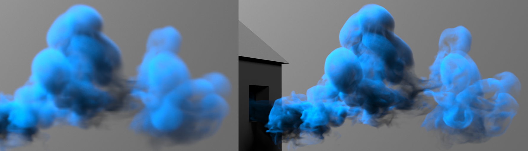
Fig. 63 GANs were shown to work well for tasks such as the inference of super-resolution solutions where the range of possible results can be highly ambiguous.#
Maximum likelihood estimation#
To train a GAN we have to briefly turn to classification problems, which we’ve managed to ignore up to now. For classification, the learning objective takes a slightly different form than the regression objective in equation (2) of Models and Equations: We now want to maximize the likelihood of a learned representation \(f\) that assigns a probability to an input \(\mathbf{x}_i\) given a set of weights \(\theta\) for a chosen set of \(i\) distinct classes. This yields a maximization problem of the form
the classic maximum likelihood estimation (MLE). In practice, it is typically turned into a sum of negative log likelihoods to give the learning objective
There are quite a few equivalent viewpoints for this fundamental expression: e.g., it can be seen as minimizing the KL-divergence between the empirical distribution as given by our training data set and the learned one. It likewise represents a maximization of the expectation as defined by the training data, i.e. \(\mathbb E \text{ log} f(\mathbf{x}_i;\theta)\). This in turn is the same as the classical cross-entropy loss for classification problems, i.e., a classifier with a sigmoid as activation function.. The takeaway message here is that the wide-spread training via cross entropy is effectively a maximum likelihood estimation for probabilities over the inputs, as defined in equation (41).
Adversarial training#
MLE is a crucial component for GANs: here we have a generator that is typically similar to a decoder network, e.g., the second half of an autoencoder from Model Reduction and Time Series. For regular GANs, the generator receives a random input vector, denoted with \(\mathbf{z}\), from which it should produce the desired output.
However, instead of directly training the generator, we employ a second network that serves as loss for the generator. This second network is called discriminator, and it has a classification task: to distinguish the generated samples from “real” ones. The real ones are typically provided in the form of a training data set, samples of which will be denoted as \(\mathbf{x}\) below.
For regular GANs training the classification task of the discriminator is typically formulated as
which, as outlined above, is a standard binary cross-entropy training for the class of real samples \(\mathbf{y}\), and the generated ones \(G(\mathbf{z})\). With the formulation above, the discriminator is trained to maximize the loss via producing an output of 1 for the real samples, and 0 for the generated ones.
The key for the generator loss is to employ the discriminator and produce samples that are classified as real by the discriminator:
Typically, this training is alternated, performing one step for \(D\) and then one for \(G\). Thus the \(D\) network is kept constant, and provides a gradient to “steer” \(G\) in the right direction to produce samples that are indistinguishable from the real ones. As \(D\) is likewise an NN, it is differentiable by construction, and can provide the necessary gradients.
Regularization#
Due to the coupled, alternating training, GAN training has a reputation of being finicky in practice. Instead of a single, non-linear optimization problem, we now have two coupled ones, for which we need to find a fragile balance. (Otherwise we’ll get the dreaded mode-collapse problem: once one of the two network “collapses” to a trivial solution, the coupled training breaks down.)
To alleviate this problem, regularization is often crucial to achieve a stable training. In the simplest case, we can add an \(L^1\) regularizer w.r.t. reference data with a small coefficient for the generator \(G\). Along those lines, pre-training the generator in a supervised fashion can help to start with a stable state for \(G\). (However, then \(D\) usually also needs a certain amount of pre-training to keep the balance.)
Conditional GANs#
For physical problems the regular GANs which generate solutions from the randomized latent-space \(\mathbf{z}\) above are not overly useful. Rather, we often have inputs such as parameters, boundary conditions or partial solutions which should be used to infer an output. Such cases represent conditional GANs, which means that instead of \(G(\mathbf{z})\), we now have \(G(\mathbf{x})\), where \(\mathbf{x}\) denotes the input data.
A good scenario for conditional GANs are super-resolution networks: These have the task to compute a high-resolution output given a sparse or low-resolution input solution.
Ambiguous solutions#
One of the main advantages of GANs is that they can prevent an undesirable averaging for ambiguous data. E.g., consider the case of super-resolution: a low-resolution observation that serves as input typically has an infinite number of possible high-resolution solutions that would fit the low-res input.
If a data set contains multiple such cases, and we employ supervised training, the network will reliably learn the mean. This averaged solution usually is one that is clearly undesirable, and unlike any of the individual solutions from which it was computed. This is the multi-modality problem, i.e. different modes existing as valid equally valid solutions to a problem. For fluids, this can, e.g., happen when we’re facing bifurcations, as discussed in A Teaser Example.
The following image shows a clear example of how well GANs can circumvent this problem:
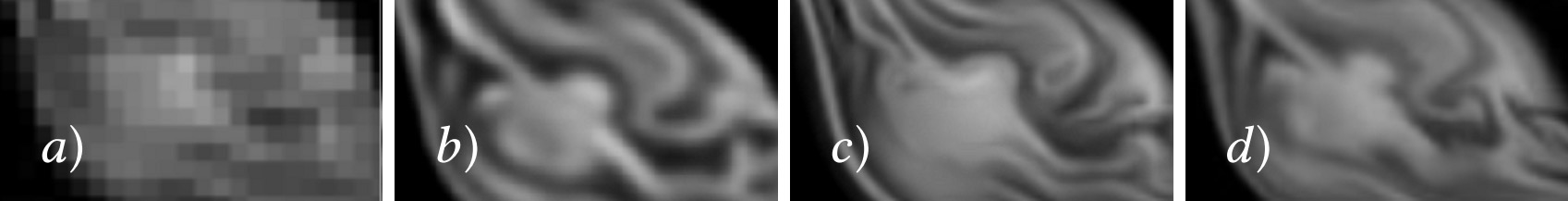
Fig. 64 A super-resolution example: a) input, b) supervised result, c) GAN result, d) high-resolution reference.#
Spatio-temporal super-resolution#
Naturally, the GAN approach is not limited to spatial resolutions. Previous work has demonstrated that the concept of learned self-supervision extends to space-time solutions, e.g., in the context of super-resolution for fluid simulations [XFCT18].
The following example compares the time derivatives of different solutions:
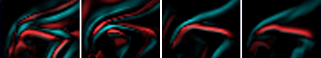
Fig. 65 From left to right, time derivatives for: a spatial GAN (i.e. not time aware), a temporally supervised learning, a spatio-temporal GAN, and a reference solution.#
As can be seen, the GAN trained with spatio-temporal self-supervision (second from right) closely matches the reference solution on the far right. In this case the discriminator receives reference solutions over time (in the form of triplets), such that it can learn to judge whether the temporal evolution of a generated solution matches that of the reference.
Physical generative models#
As a last example, GANs were also shown to be able to accurately capture solution manifolds of PDEs parametrized by physical parameters [CTS+21]. In this work, Navier-Stokes solutions parametrized by varying buoyancies, vorticity content, boundary conditions, and obstacle geometries were learned by an NN.
This is a highly challenging solution manifold, and requires an extended “cyclic” GAN approach that pushes the discriminator to take all the physical parameters under consideration into account. Interestingly, the generator learns to produce realistic and accurate solutions despite being trained purely on data, i.e. without explicit help in the form of a differentiable physics solver setup. The figure below shows a range of example outputs of a physically-parametrized GAN [CTS+21].
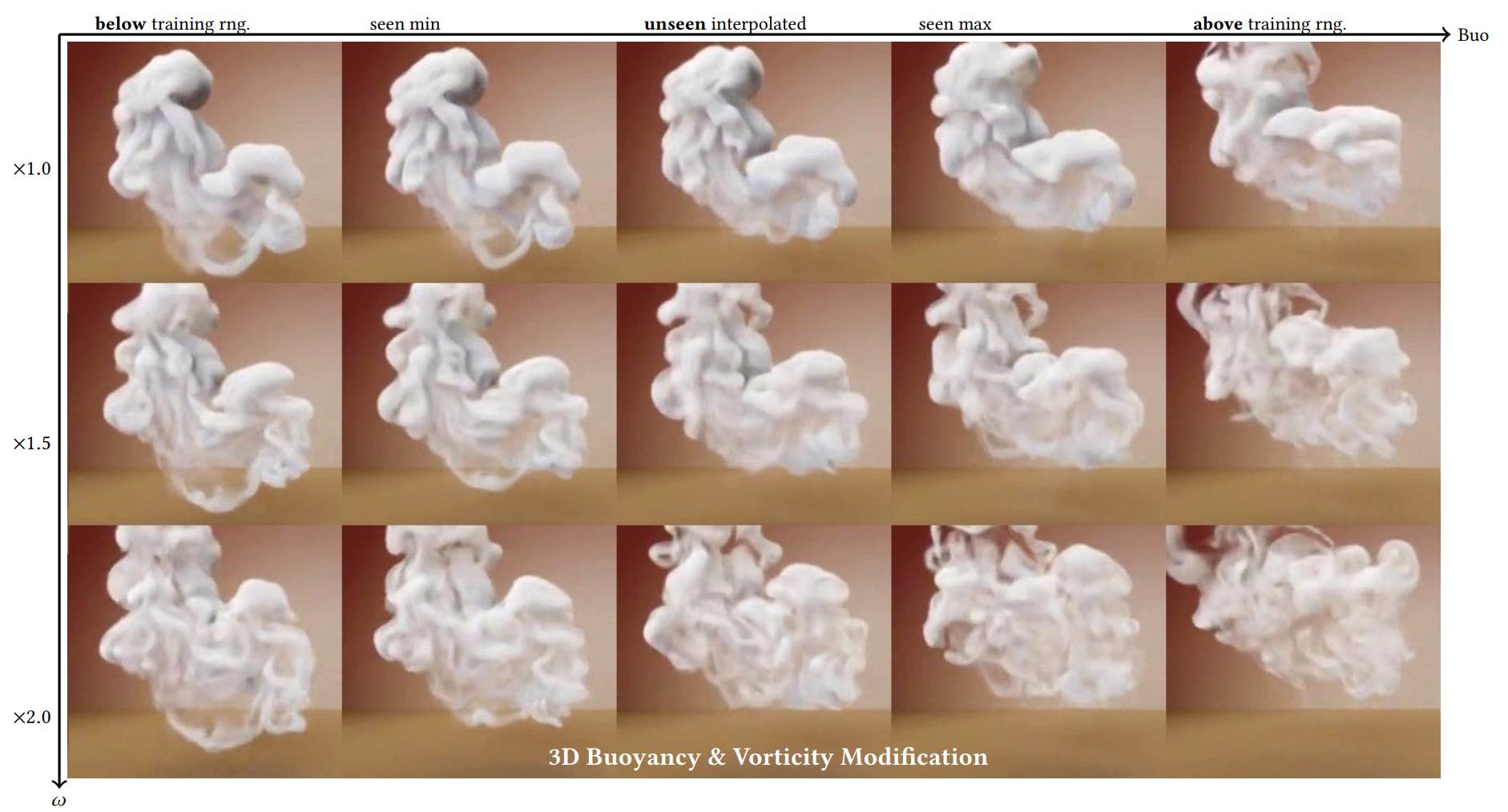
Fig. 66 The network can successfully extrapolate to buoyancy settings beyond the range of values seen at training time.#
Discussion#
GANs are a powerful learning tool. Note that the discriminator \(D\) is really “just” a learned loss function: we can completely discard it at inference time, once the generator is fully trained. Hence it’s also not overly crucial how much resources it needs.
However, despite being very powerful tools, it is (given the current state-of-the-art) questionable whether GANs make sense when we have access to a reasonable PDE model. If we can discretize the model equations and include them with a differentiable physics (DP) training (cf. Introduction to Differentiable Physics), this will most likely give better results than trying to approximate the PDE model with a discriminator. The DP training can yield similar benefits to GAN training: it yields a local gradient via the discretized simulator, and in this way prevents undesirable averaging across samples. Hence, combinations of DP training and GANs are also bound to not perform better than either of them in isolation.
That being said, GANs can nonetheless be attractive in situations where DP training is infeasible due to black-box solvers without gradients
Source code#
Due to the complexity of the training setup, we only refer to external open source implementations for practical experiments with physical GANs. E.g., the spatio-temporal GAN from [XFCT18] is available at thunil/tempoGAN.
It also includes several extensions for stabilization, such as \(L^1\) regularization, and generator-discriminator balancing.