Introduction to Reinforcement Learning#
Deep reinforcement learning, which we’ll just call reinforcement learning (RL) from now on, is a class of methods in the larger field of deep learning that takes a different viewpoint from classic “train with data” one: RL effectively lets an AI agent learn from interactions with an environment. While performing actions, the agent receives reward signals and tries to discern which actions contribute to higher rewards, to adapt its behavior accordingly. RL has been very successful at playing games such as Go [SSS+17], and it bears promise for engineering applications such as robotics.
The setup for RL generally consists of two parts: the environment and the agent. The environment receives actions \(a\) from the agent while supplying it with observations in the form of states \(s\), and rewards \(r\). The observations represent the fraction of the information from the respective environment state that the agent is able to perceive. The rewards are given by a predefined function, usually tailored to the environment and might contain, e.g., a game score, a penalty for wrong actions or a bounty for successfully finished tasks.
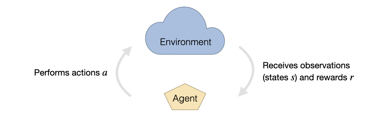
Fig. 48 Reinforcement learning is formulated in terms of an environment that gives observations in the form of states and rewards to an agent. The agent interacts with the environment by performing actions.#
In its simplest form, the learning goal for reinforcement learning tasks can be formulated as
where the reward at time \(t\) (denoted by \(r_t\) above) is the result of an action \(a\) performed by an agent. The agents choose their actions based on a neural network policy which decides via a set of given observations. The policy \(\pi(a;s, \theta)\) returns the probability for the action, and is conditioned on the state \(s\) of the environment and the weights \(\theta\).
During the learning process the central aim of RL is to uses the combined information of state, action and corresponding rewards to increase the cumulative intensity of reward signals over each trajectory. To achieve this goal, multiple algorithms have been proposed, which can be roughly divided into two larger classes: policy gradient and value-based methods [SB18].
Algorithms#
In vanilla policy gradient methods, the trained neural networks directly select actions \(a\) from environment observations. In the learning process, an NN is trained to infer the probability of actions. Here, probabilities for actions leading to higher rewards in the rest of the respective trajectories are increased, while actions with smaller return are made less likely.
Value-based methods, such as Q-Learning, on the other hand work by optimizing a state-action value function, the so-called Q-Function. The network in this case receives state \(s\) and action \(a\) to predict the average cumulative reward resulting from this input for the remainder of the trajectory, i.e. \(Q(s,a)\). Actions are then chosen to maximize \(Q\) given the state.
In addition, actor-critic methods combine elements from both approaches. Here, the actions generated by a policy network are rated based on a corresponding change in state potential. These values are given by another neural network and approximate the expected cumulative reward from the given state. Proximal policy optimization (PPO) [SWD+17] is one example from this class of algorithms and is our choice for the example task of this chapter, which is controlling Burgers’ equation as a physical environment.

Proximal policy optimization#
As PPO methods are an actor-critic approach, we need to train two interdependent networks: the actor, and the critic. The objective of the actor inherently depends on the output of the critic network (it provides feedback which actions are worth performing), and likewise the critic depends on the actions generated by the actor network (this determines which states to explore).
This interdependence can promote instabilities, e.g., as strongly over- or underestimated state values can give wrong impulses during learning. Actions yielding higher rewards often also contribute to reaching states with higher informational value. As a consequence, when the - possibly incorrect - value estimate of individual samples are allowed to unrestrictedly affect the agent’s behavior, the learning progress can collapse.
PPO was introduced as a method to specifically counteract this problem. The idea is to restrict the influence that individual state value estimates can have on the change of the actor’s behavior during learning. PPO is a popular choice especially when working on continuous action spaces. This can be attributed to the fact that it tends to achieve good results with a stable learning progress, while still being comparatively easy to implement.
PPO-clip#
More specifically, we will use the algorithm PPO-clip [SWD+17]. This PPO variant sets a hard limit for the change in behavior caused by singular update steps. As such, the algorithm uses a previous network state (denoted by a subscript \(_p\) below) to limit the change per step of the learning process. In the following, we will denote the network parameters of the actor network as \(\theta\) and those of the critic as \(\phi\).
Actor#
The actor computes a policy function returning the probability distribution for the actions conditioned by the current network parameters \(\theta\) and a state \(s\). In the following we’ll denote the probability of choosing a specific action \(a\) from the distribution with \(\pi(a; s,\theta)\). As mentioned above, the training procedure computes a certain number of weight updates using policy evaluations with a fixed previous network state \(\pi(a;s, \theta_p)\), and in intervals re-initializes the previous weights \(\theta_p\) from \(\theta\). To limit the changes, the objective function makes use of a \(\text{clip}(a,b,c)\) function, which simply returns \(a\) clamped to the interval \([b,c]\).
\(\epsilon\) defines the bound for the deviation from the previous policy. In combination, the objective for the actor is given by the following expression:
As the actor network is trained to provide the expected value, at training time an additional standard deviation is used to sample values from a Gaussian distribution around this mean. It is decreased over the course of the training, and at inference time we only evaluate the mean (i.e. a distribution with variance 0).
Critic and advantage#
The critic is represented by a value function \(V(s; \phi)\) that predicts the expected cumulative reward to be received from state \(s\). Its objective is to minimize the squared advantage \(A\):
where the advantage function \(A(s, a; \phi)\) builds upon \(V\): it’s goal is to evaluate the deviation from an average cumulative reward. I.e., we’re interested in estimating how much the decision made via \(\pi(;s,\theta_p)\) improves upon making random decisions (again, evaluated via the unchanging, previous network state \(\theta_p\)). We use the so-called Generalized Advantage Estimation (GAE) [SML+15] to compute \(A\) as:
Here \(r_t\) describes the reward obtained in time step \(t\), while \(n\) denotes the total length of the trajectory. \(\gamma\) and \(\lambda\) are two hyperparameters which influence rewards and state value predictions from the distant futures have on the advantage calculation. They are typically set to values smaller than one.
The \(\delta_t\) in the formulation above represent a biased approximation of the true advantage. Hence the GAE can be understood as a discounted cumulative sum of these estimates, from the current time step until the end of the trajectory.
Application to inverse problems#
Reinforcement learning is widely used for trajectory optimization with multiple decision problems building upon one another. However, in the context of physical systems and PDEs, reinforcement learning algorithms are likewise attractive. In this setting, they can operate in a fashion that’s similar to supervised single shooting approaches by generating full trajectories and learning by comparing the final approximation to the target.
Still, the approaches differ in terms of how this optimization is performed. For example, reinforcement learning algorithms like PPO try to explore the action space during training by adding a random offset to the actions selected by the actor. This way, the algorithm can discover new behavioral patterns that are more refined than the previous ones.
The way how long term effects of generated forces are taken into account can also differ for physical systems. In a control force estimator setup with differentiable physics (DP) loss, as discussed e.g. in Burgers Optimization with a Differentiable Physics Gradient, these dependencies are handled by passing the loss gradient through the simulation step back into previous time steps. Contrary to that, reinforcement learning usually treats the environment as a black box without gradient information. When using PPO, the value estimator network is instead used to track the long term dependencies by predicting the influence any action has for the future system evolution.
Working with Burgers’ equation as physical environment, the trajectory generation process can be summarized as follows. It shows how the simulation steps of the environment and the neural network evaluations of the agent are interleaved:
The \(*\) superscript (as usual) denotes a reference or target quantity, and hence here \(\mathbf{u}^*\) denotes a velocity target. For the continuous action space of the PDE, \(\pi\) directly computes an action in terms of a force, rather than probabilities for a discrete set of different actions.
The reward is calculated in a similar fashion as the Loss in the DP approach: it consists of two parts, one of which amounts to the negative square norm of the applied forces and is given at every time step. The other part adds a punishment proportional to the \(L^2\) distance between the final approximation and the target state at the end of each trajectory.

Implementation#
In the following, we’ll describe a way to implement a PPO-based RL training for physical systems. This implementation is also the basis for the notebook of the next section, i.e., Controlling Burgers’ Equation with Reinforcement Learning. While this notebook provides a practical example, and an evaluation in comparison to DP training, we’ll first give a more generic overview below.
To train a reinforcement learning agent to control a PDE-governed system, the physical model has to be formalized as an RL environment. The stable-baselines3 framework, which we use in the following to implement a PPO training, uses a vectorized version of the OpenAI gym environment. This way, rollout collection can be performed on multiple trajectories in parallel for better resource utilization and wall time efficiency.
Vectorized environments require a definition of observation and action spaces, meaning the in- and output spaces of the agent policy. In our case, the former consists of the current physical states and the goal states, e.g., velocity fields, stacked along their channel dimension. Another channel is added for the elapsed time since the start of the simulation divided by the total trajectory length. The action space (the output) encompasses one force value for each cell of the velocity field.
The most relevant methods of vectorized environments are reset, step_async, step_wait and render. The first of these is used to start a new trajectory by computing initial and goal states and returning the first observation for each vectorized instance. As these instances in other applications are not bound to finish trajectories synchronously, reset has to be called from within the environment itself when entering a terminal state. step_async and step_wait are the two main parts of the step method, which takes actions, applies them to the velocity fields and performs one iteration of the physics models. The split into async and wait enables supporting vectorized environments that run each instance on separate threads. However, this is not required in our approach, as phiflow handles the simulation of batches internally. The render method is called to display training results, showing reconstructed trajectories in real time or rendering them to files.
Because of the strongly differing output spaces of the actor and critic networks, we use different architectures for each of them. The network yielding the actions uses a variant of the network architecture from Holl et al. [HKT19], in line with the \(CFE\) function performing actions there. The other network consists of a series of convolutions with kernel size 3, each followed by a max pooling layer with kernel size 2 and stride 2. After the feature maps have been downsampled to one value in this way, a final fully connected layer merges all channels, generating the predicted state value.
In the example implementation of the next chapter, the BurgersTraining class manages all aspects of this training internally, including the setup of agent and environment and storing trained models and monitor logs to disk. It also includes a variant of the Burgers’ equation environment described above, which, instead of computing random trajectories, uses data from a predefined set. During training, the agent is evaluated in this environment in regular intervals to be able to compare the training progress to the DP method more accurately.
The next chapter will use this BurgersTraining class to run a full PPO scenario, evaluate its performance, and compare it to an approach that uses more domain knowledge of the physical system, i.e., the gradient-based control training with a DP approach.