Welcome …#

Welcome to the Physics-based Deep Learning Book (v0.3, the GenAI edition) 👋
TL;DR: This document is a hands-on, comprehensive guide to deep learning in the realm of physical simulations. Rather than just theory, we emphasize practical application: every concept is paired with interactive Jupyter notebooks to get you up and running quickly. Beyond traditional supervised learning, we dive into physical loss-constraints, differentiable simulations, diffusion-based approaches for probabilistic generative AI, as well as reinforcement learning and advanced neural network architectures. These foundations are paving the way for the next generation of scientific foundation models. We are living in an era of rapid transformation. These methods have the potential to redefine what’s possible in computational science.
Note
What’s new in v0.3? This latest edition adds a major new chapter on generative modeling, covering powerful techniques like denoising, flow-matching, autoregressive learning, physics-integrated constraints, and diffusion-based graph networks. We’ve also introduced a dedicated section on neural architectures specifically designed for physics simulations. All code examples have been updated to leverage the latest frameworks.
Coming up#
As a sneak preview, the next chapters will show:
How to train neural networks to predict the fluid flow around airfoils with diffusion modeling. This gives a probabilistic surrogate model that replaces and outperforms traditional simulators.
How to use model equations as residuals to train networks that represent solutions, and how to improve upon these residual constraints by using differentiable simulations.
How to more tightly interact with a full simulator for inverse problems. E.g., we’ll demonstrate how to circumvent the convergence problems of standard reinforcement learning techniques by leveraging simulators in the training loop.
We’ll also discuss the importance of choosing the right network architecture: whether to consider global or local interactions, continuous or discrete representations, and structured versus unstructured graph meshes.
Throughout this text, we will introduce different approaches for introducing physical models into deep learning, i.e., physics-based deep learning (PBDL) approaches. These algorithmic variants will be introduced in order of increasing tightness of the integration, and the pros and cons of the different approaches will be discussed. It’s important to know in which scenarios each of the different techniques is particularly useful.
Executable code, right here, right now
We focus on Jupyter notebooks, a key advantage of which is that all code examples can be executed on the spot, from your browser. You can modify things and immediately see what happens – give it a try by [running this teaser example in your browser].
Plus, Jupyter notebooks are great because they’re a form of literate programming.
Thanks!#
This project would not have been possible without the help of the many people who contributed to it. A big thanks to everyone 🙏 Here’s an alphabetical list:
Additional thanks go to Li-Wei Chen, Xin Luo, Maximilian Mueller, Chloe Paillard, Kiwon Um, and all github contributors!
Citation#
If you find this book useful, please cite it via:
@book{thuerey2021pbdl,
  title={Physics-based Deep Learning},
  author={N. Thuerey and B. Holzschuh  and P. Holl  and G. Kohl  and M. Lino  and Q. Liu and P. Schnell  and F. Trost},
  url={https://physicsbaseddeeplearning.org},
  year={2021},
  publisher={WWW}
}
Time to get started#
The future of simulation is being rewritten, and with the following AI and deep learning techniques, you’ll be at the forefront of these developments. Let’s dive in!

Comments and suggestions#
This book, where “book” stands for a collection of digital texts and code examples, is maintained by the Physics-based Simulation Group at TUM. Feel free to contact us if you have any comments, e.g., via old fashioned email. If you find mistakes, please also let us know! We’re aware that this document is far from perfect, and we’re eager to improve it. Thanks in advance 😀! Btw., we also maintain a link collection with recent research papers.
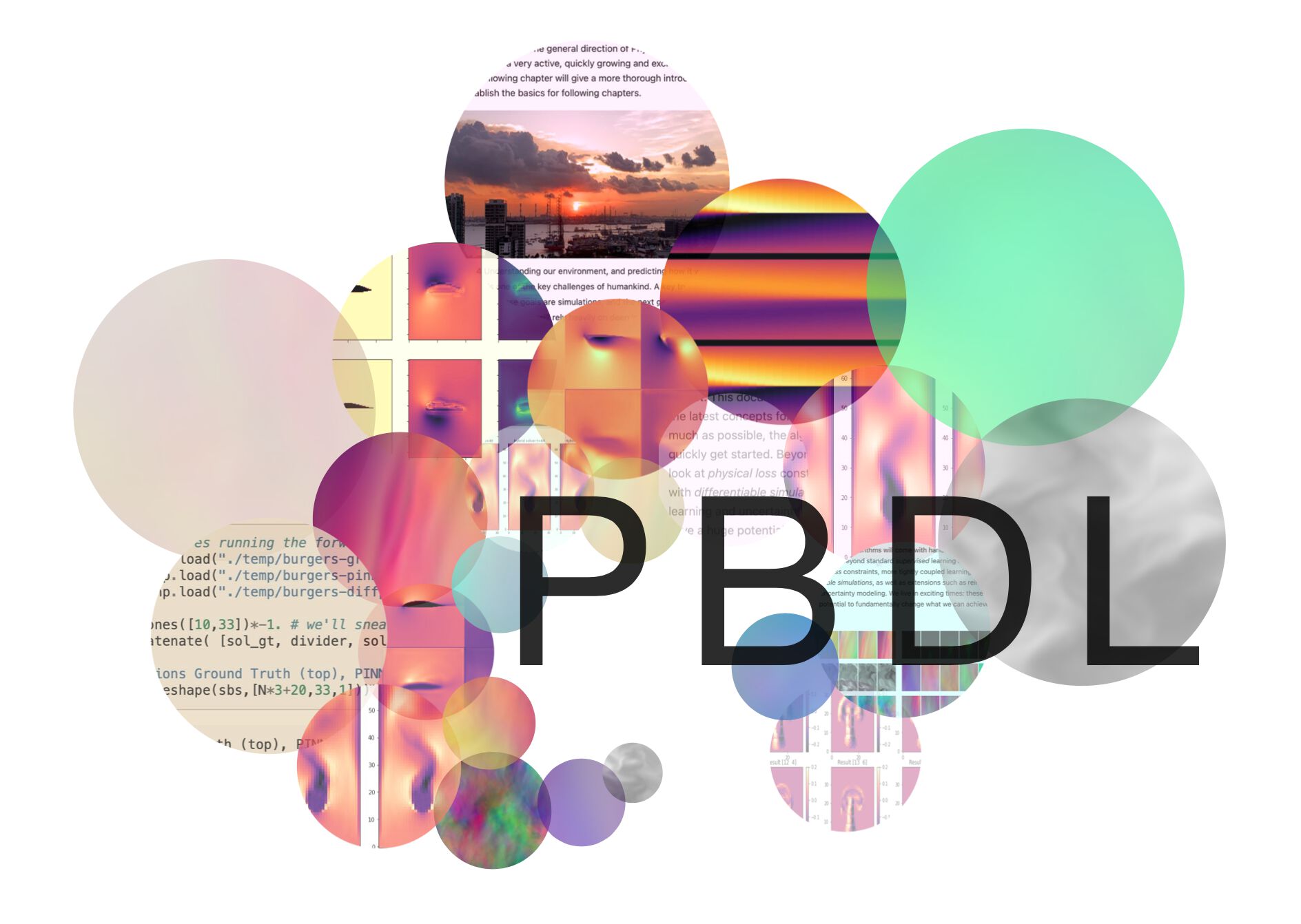
Fig. 1 Some visual examples of numerically simulated time sequences. In this book, we explain how to realize algorithms that use neural networks alongside numerical solvers.#